Function translation

There are two parts to dbplyr SQL translation: translating dplyr verbs, and translating expressions within those verbs. This vignette describes how individual expressions (function calls) are translated; vignette("translation-verb") describes how entire verbs are translated.

library(dbplyr)
library(dplyr, warn.conflicts = FALSE)

Getting started with translations

In this vignette, I’ll use lazy_frame() to create a toy lazy table that allows us to see the translation without needing to connect to a real database:

lf <- lazy_frame(x = 1, y = 2, g = "a")
lf |> mutate(z = (x + y) / 2)
#> <SQL>
#> SELECT "df".*, ("x" + "y") / 2.0 AS "z"
#> FROM "df"

The default lazy_frame() uses a generic database that generates (approximately) SQL-92 compliant SQL. You can use simulate_*() connections to see the translations used by different backends. Different databases generate slightly different SQL; see vignette("new-backend") for more details.

lf_sqlite <- lazy_frame(x = 1, con = simulate_sqlite())
lf_access <- lazy_frame(x = 1, con = simulate_access())

lf_sqlite |> transmute(z = x^2)
#> <SQL>
#> SELECT POWER(`x`, 2.0) AS `z`
#> FROM `df`
lf_access |> transmute(z = x^2)
#> <SQL>
#> SELECT "x" ^ 2.0 AS "z"
#> FROM "df"

One key difference between dbplyr-generated SQL and hand-written SQL is that dbplyr always quotes all table and column names. This is verbose but necessary because column names in database tables can be any string, including SQL reserved words like select or if. Quoting all names ensures that dbplyr-generated SQL always works regardless of the table and column names involved.

In general, perfect translation is not possible because databases don’t have all the functions that R does. The goal of dbplyr is to provide a semantic rather than a literal translation: what you mean, rather than precisely what is done. In fact, even for functions that exist both in databases and in R, you shouldn’t expect results to be identical; database programmers have different priorities than R core programmers. For example, in R in order to get a higher level of numerical accuracy, mean() loops through the data twice. R’s mean() also provides a trim option for computing trimmed means; this is something that databases do not provide.

If you’re interested in how translate_sql() is implemented, the basic techniques that underlie the implementation of translate_sql() are described in “Advanced R”.

Basic differences

There are two fundamental differences between R and SQL:

" and ' mean different things. R can use either " or ' for strings, but in ANSI SQL, must be " used for names and must be ' used for strings.
```
lf |> filter(x == "x")
#> <SQL>
#> SELECT "df".*
#> FROM "df"
#> WHERE ("x" = 'x')
```

R and SQL have different defaults for integers and reals. In R, 1 is a real, and 1L is an integer. In SQL, 1 is an integer, and 1.0 is a real.

lf |> transmute(z = 1)
#> <SQL>
#> SELECT 1.0 AS "z"
#> FROM "df"
lf |> transmute(z = 1L)
#> <SQL>
#> SELECT 1 AS "z"
#> FROM "df"

Known functions

Mathematics

basic math operators: +, -, *, /, ^
trigonometry: acos(), asin(), atan(), atan2(), cos(), cot(), tan(), sin()
hyperbolic: cosh(), coth(), sinh(), tanh()
logarithmic: log(), log10(), exp()
misc: abs(), ceiling(), floor(), sqrt(), sign(), round()

lf |> transmute(x = x / 2, y = x^2 + y^2)
#> <SQL>
#> SELECT "x", (POWER("x", 2.0)) + POWER("y", 2.0) AS "y"
#> FROM (
#>   SELECT "x" / 2.0 AS "x", "y", "g"
#>   FROM "df"
#> ) AS "q01"

lf |> transmute(x = log(x), y = round(y, 1))
#> <SQL>
#> SELECT LN("x") AS "x", ROUND("y", 1) AS "y"
#> FROM "df"

Modulo arithmetic

dbplyr translates %% to the SQL equivalents but note that it’s not precisely the same: most databases use truncated division where the modulo operator takes the sign of the dividend, where R using the mathematically preferred floored division with the modulo sign taking the sign of the divisor.

df <- tibble(
  x = c(10L, 10L, -10L, -10L),
  y = c(3L, -3L, 3L, -3L)
)
db <- copy_to(memdb(), df)

df |> mutate(x %% y)
#> # A tibble: 4 × 3
#>       x     y `x%%y`
#>   <int> <int>  <int>
#> 1    10     3      1
#> 2    10    -3     -2
#> 3   -10     3      2
#> 4   -10    -3     -1
db |> mutate(x %% y)
#> # A query:  ?? x 3
#> # Database: sqlite 3.51.1 [:memory:]
#>       x     y `x%%y`
#>   <int> <int>  <int>
#> 1    10     3      1
#> 2    10    -3      1
#> 3   -10     3     -1
#> 4   -10    -3     -1

dbplyr no longer translates %/% because there’s no robust cross-database translation available.

Logical comparisons and boolean operations

logical comparisons: <, <=, !=, >=, >, ==, %in%, between()
boolean operations: &, &&, |, ||, !, xor()

lf |> filter(x > 5 | y == 2)
#> <SQL>
#> SELECT "df".*
#> FROM "df"
#> WHERE ("x" > 5.0 OR "y" = 2.0)

lf |> filter(x %in% c(1, 2, 3))
#> <SQL>
#> SELECT "df".*
#> FROM "df"
#> WHERE ("x" IN (1.0, 2.0, 3.0))

lf |> filter(between(x, 1, 5))
#> <SQL>
#> SELECT "df".*
#> FROM "df"
#> WHERE ("x" BETWEEN 1.0 AND 5.0)

Bitwise operations

bitwNot(), bitwAnd(), bitwOr(), bitwXor(), bitwShiftL(), and bitwShiftR() are all supported:

lf |> transmute(x = bitwAnd(x, 3L), y = bitwShiftL(x, 2L))
#> <SQL>
#> SELECT "x", "x" << 2 AS "y"
#> FROM (
#>   SELECT "x" & 3 AS "x", "y", "g"
#>   FROM "df"
#> ) AS "q01"

Type coercion

Type coercion functions use the corresponding SQL CAST() call:

lf |> transmute(x = as.integer(y), y = as.character(x))
#> <SQL>
#> SELECT "x", CAST("x" AS TEXT) AS "y"
#> FROM (
#>   SELECT CAST("y" AS INTEGER) AS "x", "y", "g"
#>   FROM "df"
#> ) AS "q01"

integer types: as.integer(), as.integer64()
floating point: as.numeric(), as.double()
character: as.character()
logical: as.logical()
date/time: as.Date(), as.POSIXct()

`NULL`/`NA` handling

is.na(), is.null(): test for NULL.
na_if(): replace a value with NULL.
coalesce(): replace NULL with a default value.

lf |> filter(!is.na(x))
#> <SQL>
#> SELECT "df".*
#> FROM "df"
#> WHERE (NOT(("x" IS NULL)))

lf |> transmute(x = coalesce(x, 0L))
#> <SQL>
#> SELECT COALESCE("x", 0) AS "x"
#> FROM "df"

lf |> transmute(x = na_if(x, 0L))
#> <SQL>
#> SELECT NULLIF("x", 0) AS "x"
#> FROM "df"

Aggregation

All databases provide translation for the basic aggregations: mean(), sum(), min(), max(). Databases automatically drop NULLs (their equivalent of missing values) whereas in R you have to ask nicely. The aggregation functions warn you about this important difference:

lf |> summarise(z = mean(x))
#> Warning: Missing values are always removed in SQL aggregation functions.
#> Use `na.rm = TRUE` to silence this warning
#> This warning is displayed once every 8 hours.
#> <SQL>
#> SELECT AVG("x") AS "z"
#> FROM "df"
lf |> summarise(z = mean(x, na.rm = TRUE))
#> <SQL>
#> SELECT AVG("x") AS "z"
#> FROM "df"

Note that aggregation functions used inside mutate() or filter() generate a window translation:

lf |> mutate(z = mean(x, na.rm = TRUE))
#> <SQL>
#> SELECT "df".*, AVG("x") OVER () AS "z"
#> FROM "df"
lf |> filter(mean(x, na.rm = TRUE) > 0)
#> <SQL>
#> SELECT "x", "y", "g"
#> FROM (
#>   SELECT "df".*, AVG("x") OVER () AS "col01"
#>   FROM "df"
#> ) AS "q01"
#> WHERE ("col01" > 0.0)

Most backends also support:

sd(), var(), cor(), cov()
median(), quantile()
n(), n_distinct()
all(), any()
str_flatten()

Conditional evaluation

if, ifelse(), and if_else() are translated to CASE WHEN:

lf |> transmute(z = ifelse(x > 5, "big", "small"))
#> <SQL>
#> SELECT CASE WHEN ("x" > 5.0) THEN 'big' WHEN NOT ("x" > 5.0) THEN 'small' END AS "z"
#> FROM "df"

case_when(), case_match(), and switch() are also supported:

lf |> 
  mutate(z = case_when(
    x > 10 ~ "medium",
    x > 30 ~ "big", 
    .default = "small"
  ))
#> <SQL>
#> SELECT
#>   "df".*,
#>   CASE
#> WHEN ("x" > 10.0) THEN 'medium'
#> WHEN ("x" > 30.0) THEN 'big'
#> ELSE 'small'
#> END AS "z"
#> FROM "df"

lf |> mutate(z = switch(g, a = 1L, b = 2L, 3L))
#> <SQL>
#> SELECT
#>   "df".*,
#>   CASE "g" WHEN ('a') THEN (1) WHEN ('b') THEN (2) ELSE (3) END AS "z"
#> FROM "df"

String functions

Base R string functions and their stringr equivalents are widely supported:

nchar(), str_length()
tolower(), toupper(), str_to_lower(), str_to_upper(), str_to_title()
trimws(), str_trim()
paste(), paste0(), str_c()
substr(), substring(), str_sub()

lf |> transmute(x = paste0(g, " dog"))
#> <SQL>
#> SELECT CONCAT_WS('', "g", ' dog') AS "x"
#> FROM "df"

lf |> transmute(x = substr(g, 1L, 2L))
#> <SQL>
#> SELECT SUBSTR("g", 1, 2) AS "x"
#> FROM "df"

Many backends also support regular expression functions like str_detect(), str_replace(), str_replace_all(), str_remove(), str_remove_all(), str_squish(), and str_like(). Support varies by backend; see the individual backend documentation for details.

Date/time functions

dbplyr supports many lubridate functions for extracting date components:

today(), now()
year(), month(), day(), mday(), hour(), minute(), second()

lf_dt <- lazy_frame(dt = Sys.time())

lf_dt |> transmute(
  year = year(dt),
  month = month(dt),
  day = day(dt)
)
#> <SQL>
#> SELECT
#>   EXTRACT(year FROM "dt") AS "year",
#>   EXTRACT(month FROM "dt") AS "month",
#>   EXTRACT(day FROM "dt") AS "day"
#> FROM "df"

Some backends also support additional lubridate functions including yday(), wday(), week(), isoweek(), quarter(), isoyear(), floor_date(), and period functions like seconds(), minutes(), hours(), days(), weeks(), months(), years().

Several backends (including PostgreSQL, Snowflake, SQL Server, Redshift, and Spark SQL) support clock functions for date arithmetic.

add_days(), add_years()
date_build()
get_year(), get_month(), get_day()
date_count_between()
difftime()

clock functions tend to be easier to translate than lubridate functions because they are more specific.

Other functions

pmin(), pmax() for parallel min/max
desc() for descending order
cut() for binning numeric values into categories

Unknown functions

Any function that dbplyr doesn’t know how to convert is left as is. This means that database functions that are not covered by dbplyr can often be used directly.

Prefix functions

Any function that dbplyr doesn’t know about will be left as is:

lf |> mutate(z = foofify(x, y))
#> <SQL>
#> SELECT "df".*, foofify("x", "y") AS "z"
#> FROM "df"

But to make it clear that you’re deliberately calling a SQL function, we recommend using the .sql pronoun:

lf |> transmute(z = .sql$foofify(x, y))
#> <SQL>
#> SELECT foofify("x", "y") AS "z"
#> FROM "df"

If you’re working inside a package, this also makes it easier to avoid R CMD CHECK notes. Just import .sql from dbplyr using a roxygen2 tag like @importFrom dbplyr .sql

Infix functions

As well as prefix functions (where the name of the function comes before the arguments), dbplyr also translates infix functions. That allows you to use expressions like LIKE, which does a limited form of pattern matching:

lf |> filter(x %LIKE% "%foo%")
#> <SQL>
#> SELECT "df".*
#> FROM "df"
#> WHERE ("x" LIKE '%foo%')

You can also use str_like() for this common case:

lf |> filter(str_like(x, "%foo%"))
#> <SQL>
#> SELECT "df".*
#> FROM "df"
#> WHERE ("x" LIKE '%foo%')

You could use %||% for string concatenation, but in most cases it’s more R-like to use paste() or paste0():

lf |> transmute(z = x %||% y)
#> <SQL>
#> SELECT "x" || "y" AS "z"
#> FROM "df"
lf |> transmute(z = paste0(x, y))
#> <SQL>
#> SELECT CONCAT_WS('', "x", "y") AS "z"
#> FROM "df"
lf |> transmute(z = paste(x, y))
#> <SQL>
#> SELECT CONCAT_WS(' ', "x", "y") AS "z"
#> FROM "df"

Special forms

SQL functions tend to have a greater variety of syntax than R. That means there are a number of expressions that can’t be translated directly from R code. To insert these in your own queries, you can use literal SQL inside sql():

lf |> transmute(z = sql("x!"))
#> <SQL>
#> SELECT x! AS "z"
#> FROM "df"
lf |> transmute(z = x == sql("ANY VALUES(1, 2, 3)"))
#> <SQL>
#> SELECT "x" = ANY VALUES(1, 2, 3) AS "z"
#> FROM "df"

This gives you a lot of freedom to generate the SQL you need:

lf |> transmute(factorial = sql("x!"))
#> <SQL>
#> SELECT x! AS "factorial"
#> FROM "df"
lf |> transmute(factorial = sql("CAST(x AS FLOAT)"))
#> <SQL>
#> SELECT CAST(x AS FLOAT) AS "factorial"
#> FROM "df"

Error for unknown translations

If needed, you can also use the dplyr.strict_sql option to force dbplyr to error if it doesn’t know how to translate a function:

options(dplyr.strict_sql = TRUE)
lf |> mutate(z = glob(x, y))
#> Error in `glob()`:
#> ! Don't know how to translate `glob()`

Window functions

Things get a little trickier with window functions, because SQL’s window functions are considerably more expressive than the specific variants provided by base R or dplyr. They have the form [expression] OVER ([partition clause] [order clause] [frame_clause]):

The expression is a combination of variable names and window functions. Support for window functions varies from database to database, but most support:
- ranking: row_number(), min_rank(), rank(), dense_rank(), percent_rank(), cume_dist(), ntile();
- offsets: lead(), lag(), first(), last(), nth();
- aggregates: mean(), sum(), min(), max(), n(), n_distinct();
- cumulative: cummean(), cumsum(), cummin(), cummax().
The partition clause specifies how the window function is broken down over groups. It plays an analogous role to GROUP BY for aggregate functions, and group_by() in dplyr. It is possible for different window functions to be partitioned into different groups, but not all databases support it, and neither does dplyr.
The order clause controls the ordering (when it makes a difference). This is important for the ranking functions since it specifies which variables to rank by, but it’s also needed for cumulative functions and lead. Whenever you’re thinking about before and after in SQL, you must always tell it which variable defines the order. If the order clause is missing when needed, some databases fail with an error message while others return non-deterministic results.
The frame clause defines which rows, or frame, that are passed to the window function, describing which rows (relative to the current row) should be included. The frame clause provides two offsets which determine the start and end of frame. There are three special values: -Inf means to include all preceding rows (in SQL, “unbounded preceding”), 0 means the current row (“current row”), and Inf means all following rows (“unbounded following”). The complete set of options is comprehensive, but fairly confusing, and is summarised visually below.

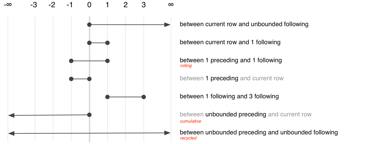
Of the many possible specifications, only three are commonly used. They select between aggregation variants:
- Recycled: BETWEEN UNBOUND PRECEDING AND UNBOUND FOLLOWING
- Cumulative: BETWEEN UNBOUND PRECEDING AND CURRENT ROW
- Rolling: BETWEEN 2 PRECEDING AND 2 FOLLOWING
dbplyr generates the frame clause based on whether you’re using a recycled aggregate or a cumulative aggregate.

To see how individual window functions are translated to SQL, we can use transmute():

lf <- lazy_frame(g = 1, year = 2020, id = 3, con = simulate_dbi())

lf |> transmute(
  mean = mean(g), 
  rank = min_rank(g), 
  cumsum = cumsum(g),
  lag = lag(g)
)
#> Warning: Windowed expression `SUM("g")` does not have explicit order.
#> ℹ Please use `arrange()`, `window_order()`, or `.order` to make
#>   deterministic.
#> <SQL>
#> SELECT
#>   AVG("g") OVER () AS "mean",
#>   CASE
#> WHEN (NOT(("g" IS NULL))) THEN RANK() OVER (PARTITION BY (CASE WHEN (("g" IS NULL)) THEN 1 ELSE 0 END) ORDER BY "g")
#> END AS "rank",
#>   SUM("g") OVER (ROWS UNBOUNDED PRECEDING) AS "cumsum",
#>   LAG("g", 1, NULL) OVER () AS "lag"
#> FROM "df"

If the lazy frame has been grouped or arranged previously in the pipeline, then dbplyr will use that information to set the “partition by” and “order by” clauses:

lf |> arrange(year) |> mutate(z = cummean(g))
#> <SQL>
#> SELECT "df".*, AVG("g") OVER (ORDER BY "year" ROWS UNBOUNDED PRECEDING) AS "z"
#> FROM "df"
#> ORDER BY "year"
lf |> group_by(id) |> mutate(z = rank())
#> <SQL>
#> SELECT "df".*, RANK() OVER (PARTITION BY "id") AS "z"
#> FROM "df"

There are some challenges when translating window functions between R and SQL, because dbplyr tries to keep the window functions as similar as possible to both the existing R analogues and to the SQL functions. This means that there are three ways to control the order clause depending on which window function you’re using:

For ranking functions, the ordering variable is the first argument: rank(x), ntile(y, 2). If omitted or NULL, will use the default ordering associated with the tbl (as set by arrange()).
Accumulating aggregates only take a single argument (the vector to aggregate). To control ordering, use order_by().
Aggregates implemented in dplyr (lead(), lag(), nth(), first(), last()) have an order_by argument. Supply it to override the default ordering.

The three options are illustrated in the snippet below:

lf |> transmute(
  x1 = min_rank(g),
  x2 = order_by(year, cumsum(g)),
  x3 = lead(g, order_by = year)
)
#> <SQL>
#> SELECT
#>   CASE
#> WHEN (NOT(("g" IS NULL))) THEN RANK() OVER (PARTITION BY (CASE WHEN (("g" IS NULL)) THEN 1 ELSE 0 END) ORDER BY "g")
#> END AS "x1",
#>   SUM("g") OVER (ORDER BY "year" ROWS UNBOUNDED PRECEDING) AS "x2",
#>   LEAD("g", 1, NULL) OVER (ORDER BY "year") AS "x3"
#> FROM "df"

Currently there is no way to order by multiple variables, except by setting the default ordering with arrange(). This will be added in a future release.